Zinc-nickel coatings - Aplikacje

Aplikacje / zinc-nickel coatings

01 — Introduction

Zinc-nickel: the high-performance sacrificial coating for steel parts

Zinc-nickel coatings are an alloy layer combining zinc (typically 84 – 88 %) and nickel (12 – 16 %). They are increasingly used to protect steel parts against corrosion: the zinc is sacrificial — it corrodes before the ferrous substrate — while the nickel slows that very process down. Where a standard zinc coating resists 96 – 120 hours in a salt-spray test, a zinc-nickel coating can last more than 1 000 hours, and remains stable at temperatures above 120 °C.

The automotive industry is one of the largest users of ZnNi, for parts exposed to the outside environment or to high temperatures: battery covers, brake systems (calipers and rotors), fasteners. In aerospace, ZnNi is increasingly adopted as a non-toxic, REACH-compliant alternative to cadmium plating on landing-gear components, electrical connectors and fasteners (bolts, nuts and screws).

Alkaline ZnNi Acid ZnNi Rack plating Barrel plating Cadmium replacement

Battery cover protected with a ZnNi coating

The electroplating process

ZnNi coatings are deposited by electroplating. The parts are immersed in a chemical bath containing zinc and nickel ions; a current is applied to the part, the ions migrate to its surface and are reduced into a zinc-nickel alloy layer, generally 8 to 15 µm thick. The layer is then passivated and often sealed with a topcoat to reach the specified corrosion performance and friction coefficient.

Figure 1 — ZnNi plating line sequence

The Enovasense measurement is possible on the bare ZnNi layer and through the passivation and topcoat, with a calibration per process state.

02 — Quality Requirements

Why thickness and uniformity are critical in a complex electroplating process

The thickness of a ZnNi coating — and its homogeneity over the part — is what guarantees the corrosion protection. But depositing too much is not an option either: an over-thick layer becomes brittle and threatens the mechanical fit of the part, particularly for fasteners in threads, where the coating directly consumes the thread tolerance.

Large parts: uneven current distribution

On a large battery cover plated on a rack, it is difficult to ensure that the electrical current is applied evenly over the whole surface. Current density concentrates on edges and protrusions and drops in recesses, which inevitably leads to an inhomogeneous deposition: thick on the edges, thin in the corners and inside the cavities.

Small parts: barrel plating in batches

Fasteners and small components are plated as batches in a rotating barrel. The electrical contact between parts is intermittent and uniformity is even harder to reach, from part to part and from head to thread on the same part.

Figure 2 — Thickness non-uniformity inherent to electroplating (schematic)

Specifications and the cost of over-plating

OEM and aerospace specifications define a minimum local thickness, a thickness range and a salt-spray target (red rust, white rust). Plating thicker than necessary to secure the local minimum wastes nickel, lengthens the cycle and increases hydrogen-embrittlement risk on high-strength steels. Measuring the distribution on the actual part — not only on a reference panel — is the only way to tune the rack design, the anode layout and the plating time.

> 1 000 h Salt-spray resistance of a ZnNi coating, against 96 – 120 h for standard zinc	8 – 15 µm Typical ZnNi thickness — a narrow window where every micron of uniformity matters
± 3 µm Maximum deviation over ± 5 mm of working distance and ± 40° of approach angle	Cg 1.69 / Cgk 1.66 Type 1 MSA gauge capability — above the 1.33 acceptance threshold

03 — Measurement Challenges

How ZnNi thickness is measured today — and where each method stops

Besides destructive cross-section microscopy and coulometric stripping, three non-destructive techniques are used in plating shops: magnetic-induction probes, handheld XRF and benchtop XRF. Each has its place — and each hits a limit where the part geometry, the throughput or the operator comes into play.

Magnetic-induction probes: fast, but contact and operator dependent

Magnetic induction measures the non-magnetic ZnNi layer on the ferromagnetic steel in one second, but it requires contact: the reading depends on how the probe is applied, needs regular recalibration, and fails close to edges and holes or on curved surfaces — exactly where the plating is the least uniform.

Handheld XRF: elemental, but slow and coarse

Handheld X-ray fluorescence reads the Zn and Ni signals near contact, in 5 to 30 seconds depending on the accuracy required. Its 3 – 8 mm spot cannot handle small parts or thread flanks, the reading drifts over time, and the result depends on the operator.

Benchtop XRF: precise, but confined to the laboratory

Benchtop XRF offers a 0.1 – 0.3 mm spot for small areas and low operator dependency, but needs 15 – 20 seconds per point, a distance tolerance of only ± 0.1 – 0.5 mm, a shielded enclosure, and still struggles close to edges and holes. It is a laboratory audit tool, not a production control.

04 — Technology Comparison

Why laser photothermal radiometry is the right fit for ZnNi

Enovasense’s patented laser photothermal radiometry measures the coating through its thermal response: a modulated laser beam heats the surface by a few degrees, the thermal wave diffuses through the ZnNi layer and reflects at the steel interface, and an infrared detector converts the phase of the returning signal into thickness. The measurement is non-contact at 40 mm with ± 3 mm tolerance, takes 1 second, uses a 1 mm spot without edge effect, is independent of the operator and does not drift — which makes it faster and more stable than contact or XRF gauges, and the natural choice for in-line integration.

Criteria	Enovasense laser photothermal	Magnetic induction probe	Handheld XRF	Benchtop XRF
Measurement principle	Thermal diffusion response	Magnetic field response	X-ray fluorescence of the coating	X-ray fluorescence of the coating
Contact and distance	Non-contact — 40 mm, ± 3 mm tolerance	Contact	Near contact	Non-contact — 20 mm, ± 0.1 – 0.5 mm tolerance
Measuring time	1 s	1 s	5 – 30 s depending on accuracy	15 – 20 s
Operator influence	Independent	Dependent — how contact is applied	Dependent	Low
Calibration	No recalibration — no drift	Regular recalibration	Drifts — regular recalibration	Drifts — regular recalibration
Size, shape and edge dependency	Independent — 1 mm spot, no edge effect	Shape dependent — not near edges and holes	Shape dependent — 3 – 8 mm spot, no small parts	Shape dependent — 0.1 – 0.3 mm spot, not near edges / holes
Automation	Yes — probe on a robot arm or fixed in line	Handheld device	Handheld device	Benchtop device

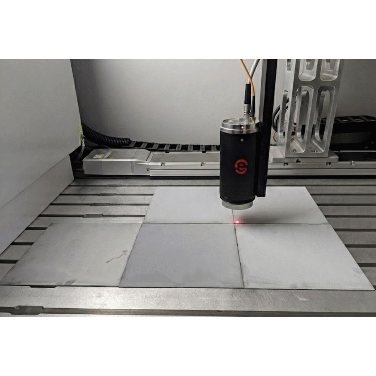
Zinc-nickel coating thickness measurement with an Enovasense sensor

05 — Metrological Performance

How Enovasense performs on ZnNi coatings

To assess accuracy, tests were performed on samples whose thicknesses cover the whole tolerance interval, between 10 and 30 µm. The Enovasense values were compared with magnetic-induction measurements on the same samples.

Figure 3 — Enovasense laser photothermal vs magnetic induction, ZnNi samples 10 – 30 µm

Mean Enovasense thickness per sample against the magnetic-induction reference. Schematic rendering of the study data.

The Enovasense sensor correlates closely with the magnetic-induction values over the whole range, with a single calibration.

Gauge capability: type 1 MSA study

A type 1 measurement system analysis was then performed on a sample with a reference thickness of 41 µm, by repeating the measurement at the same point under controlled conditions.

Figure 4 — Type 1 gauge study on a 41 µm ZnNi coating

Run chart of the repeated measurements against the reference value. Schematic rendering consistent with the study statistics.

Bias: the p-value (0.6356) is higher than the standard alpha level of 0.05 — the bias is not statistically significant. The measurement system is accurate relative to the reference.
Capability: both Cg (1.69) and Cgk (1.66) exceed the standard threshold of 1.33 — the measurement system is capable; its variation is acceptably small compared with the allocated tolerance.

Tolerance to distance and angle: the key to real parts

Finally, the influence of the measurement distance and of the approach angle was tested — the two parameters that vary constantly on curved parts, in robotic handling or in barrel-plated batches. The sensor stays within ± 3 µm when the distance varies from 15 to 25 mm (nominal 20 mm) and when the approach angle varies from −40° to +40° (nominal 0°).

Figure 5 — Measurement deviation vs working distance and approach angle

Deviation from the nominal reading as the sensor is moved away from its nominal distance and tilted around its nominal angle. Green band: ± 3 µm. Schematic rendering of the study results.

This robustness is what makes the difference between a laboratory gauge and a production sensor: a part presented by a robot, a curved caliper surface or a fastener in a tray can be measured without precise positioning and without a mechanical reference stop.

Performance figures correspond to the configurations used in these studies. Actual performance depends on the optical system selected, the ZnNi process (alkaline or acid, passivation and topcoat) and the thickness range measured. A dedicated calibration is built per process state.

06 — Industrial Integration

Integrating Enovasense sensors for ZnNi control

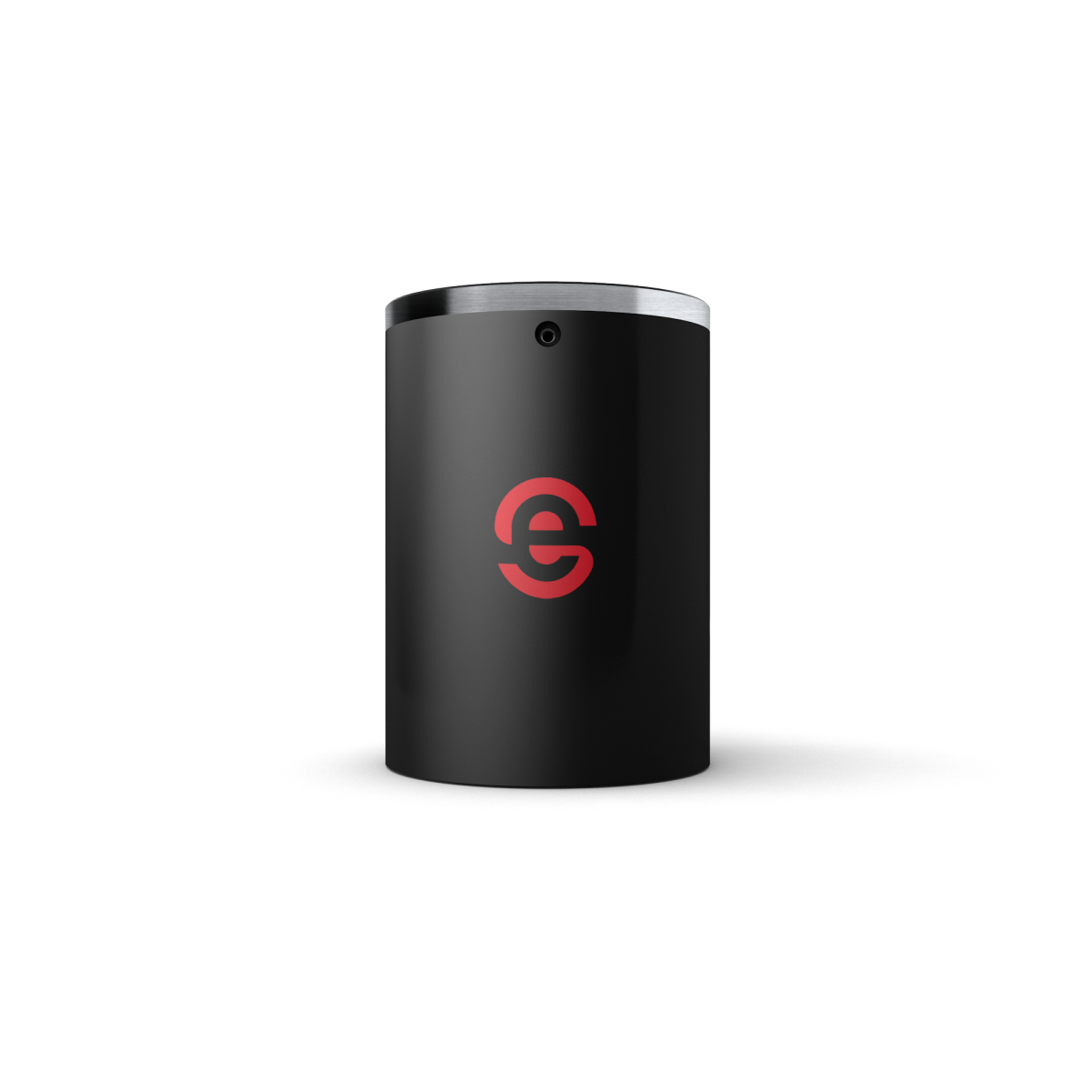
The Enovasense probes are compact and lightweight, and their tolerance to distance and angle opens several integration routes, from the plating shop laboratory to the end of the line.

Robotic integration or fixed position

The compact probe mounts on a robot arm to automatically measure a programmed set of positions on the part — edges, recesses and thread areas included. For large parts such as battery covers, the part itself can be brought by the robot to one or several sensors installed in a fixed position.

Off-line control station — HKL2

The HKL2 station performs thickness mapping and programmed cycles of movements and measurements with a 3-axis system, measuring multiple positions on a part automatically. For small parts such as fasteners, it measures batches of parts in a tray — a direct check of barrel-plating uniformity.

In-line integration

At the exit of the plating line, the sensor measures every rack or a sample of every barrel load without contact, streaming the thickness to the plant network for closed-loop control of plating time and current, and for per-batch traceability.


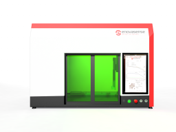Compact Enovasense probe for robotic or fixed-position integration	HKL2 off-line control station — automated mapping and batch measurement